Static Priority Preemtive Example

Introduction

In this section, we will dissect the SPP example which is representative for the ideas behind pyCPA. The full source code of the example is shown at the end of this section.

Before we begin some general reminder:

pyCPA is NOT a tool! It rather is a package of methods and classes which can be embedded into your pyhon application - the spp example is such an example application.

Each pyCPA program consists of three steps:

• initialization
• setting up the architecture
• one or multiple scheduling analyses

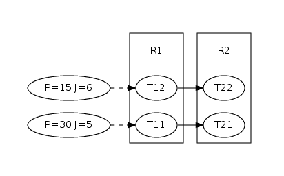
The architecture can be entered in two ways, either you provide it with the source code or you can use an XML loader such as the Symta or the SMFF loader. However, in most cases it is sufficient to code your architecture directly in a python file. For this example we assume that our architecture consists of two resources (e.g. CPUs) scheduled by an static-priority-preemptive (SPP) scheduler and four tasks of which some communicate by event-triggering. The environment stimulus (e.g. an sensor or input from another system) is assumed to be periodic with jitter. The application graph is shown on on the right.

Initialization

Now, let’s look at the example. Before we actually start with the program, we import all pycpa modules which are needed for this example

from pycpa import model
from pycpa import analysis
from pycpa import schedulers
from pycpa import graph
from pycpa import options

The interesting module are pycpa.spp which contains scheduler specific algorithms, pycpa.graph which is used to plot a task graph of this example and pycpa.options which controls various modes in which pyCPA can be executed.

pyCPA can be initialized by pycpa.options.init_pycpa(). This will parse the pyCPA related options such as the propagation method, verbosity, maximum-busy window, etc. Conveniently, this also prints the options which will be used for your pyCPA session. This is handy, when you run some analyses in batch jobs and want are uncertain about the exact settings after a few weeks. However, the explicit call of this function is not necessary most of the time, as it is being implicitly called at the beginning of the analysis. It can be useful to control the exact time where the initialization happens in case you want to manually override some options from your code.

System Model

Now, we create an empty system, which is just a container for all other objects:

    # generate an new system
    s = model.System()

The next step is to create two resources R1 and R2 and bind them to the system via pycpa.model.System.bind_resource(). When creating a resource via pycpa.model.Resource(), the first argument of the constructor sets the resource id (a string) and the second defines the scheduling policy. The scheduling policy is defined by a reference to an instance of a scheduler class derived from pycpa.analysis.Scheduler. For SPP, this is pycpa.spp.SPPScheduler. In this class, different functions are defined which for instance compute the multiple-event busy window on that resource or the stopping condition for that particular scheduling policy. The stopping condition specifies how many activations of a task have to be considered for the analysis. The default implementations of these functions from pycpa.analysis.Scheduler can be used for certain schedulers, but generally should be overridden by scheduler-specific versions. For SPP we have to look at all activations which fall in the level-i busy window, thus we choose the spp stopping condition.

    r1 = s.bind_resource(model.Resource("R1", schedulers.SPPScheduler()))
    r2 = s.bind_resource(model.Resource("R2", schedulers.SPPScheduler()))

The next part is to create tasks via pycpa.model.Resource() and bind them to a resource via pycpa.model.Resource.bind_task(). For tasks, we pass some parameters to the constructor, namely the identifier (string), the scheduling_paramter denoting the priority, and the worst- and best-case execution times (wcet and bcet).

    # create and bind tasks to r1
    t11 = r1.bind_task(model.Task("T11", wcet=10, bcet=5, scheduling_parameter=1))
    t12 = r1.bind_task(model.Task("T12", wcet=3, bcet=1, scheduling_parameter=2))

    # create and bind tasks to r2
    t21 = r2.bind_task(model.Task("T21", wcet=2, bcet=2, scheduling_parameter=1))
    t22 = r2.bind_task(model.Task("T22", wcet=9, bcet=4, scheduling_parameter=2))

In case tasks communicate with each other through event propagation (e.g. one task fills the queue of another task), we model this through task links, which are created by pycpa.model.Task.link_dependent_task() A task link is abstract and does not consume any additional time. In case of communication-overhead it must be modeled by using other resources/tasks.

    # specify precedence constraints: T11 -> T21; T12-> T22
    t11.link_dependent_task(t21)
    t12.link_dependent_task(t22)

Lastly we must set the input event models for all tasks that are not activated by another task. An event model is an abstraction of possible activation patterns and are commonly parametrized by an activation period P, a jitter J (optional) and an minimum distance d (optional). Such an event model is created by pycpa.model.PJdEventModel.

    # register a periodic with jitter event model for T11 and T12
    t11.in_event_model = model.PJdEventModel(P=30, J=5)
    t12.in_event_model = model.PJdEventModel(P=15, J=6)

Plotting the Task-Graph

Then, we plot the taskgraph to a pdf file by using pycpa.graph.graph_system() from the graph module.

    # plot the system graph to visualize the architecture
    g = graph.graph_system(s, 'spp_graph.pdf', dotout='spp_graph.dot')

Analysis

The analysis is performed by calling pycpa.analysis.analyze_system(). This will will find the fixed-point of the scheduling problem and terminate if a result was found or if the system is not feasible (e.g. one busy window or the amount a propagations was larger than a limit or the load on a resource is larger one).

    # perform the analysis
    print("Performing analysis")
    task_results = analysis.analyze_system(s)

pycpa.analysis.analyze_system() returns a dictionary with results for each task in the form of instances to pycpa.analysis.TaskResult. Finally, we print out some of the results:

    # print the worst case response times (WCRTs)
    print("Result:")
    for r in sorted(s.resources, key=str):
        for t in sorted(r.tasks, key=str):
            print("%s: wcrt=%d" % (t.name, task_results[t].wcrt))

The output of this example is:

pyCPA - Compositional Performance Analysis in Python.

Version 1.2
Copyright (C) 2010-2017, TU Braunschweig, Germany. All rights reserved.

Permission is hereby granted, free of charge, to any person obtaining a copy
of this software and associated documentation files (the "Software"), to deal
in the Software without restriction, including without limitation the rights
to use, copy, modify, merge, publish, distribute, sublicense, and/or sell
copies of the Software, and to permit persons to whom the Software is
furnished to do so, subject to the following conditions:

The above copyright notice and this permission notice shall be included in
all copies or substantial portions of the Software.

THE SOFTWARE IS PROVIDED "AS IS", WITHOUT WARRANTY OF ANY KIND, EXPRESS OR
IMPLIED, INCLUDING BUT NOT LIMITED TO THE WARRANTIES OF MERCHANTABILITY,
FITNESS FOR A PARTICULAR PURPOSE AND NONINFRINGEMENT. IN NO EVENT SHALL THE
AUTHORS OR COPYRIGHT HOLDERS BE LIABLE FOR ANY CLAIM, DAMAGES OR OTHER
LIABILITY, WHETHER IN AN ACTION OF CONTRACT, TORT OR OTHERWISE, ARISING FROM,
OUT OF OR IN CONNECTION WITH THE SOFTWARE OR THE USE OR OTHER DEALINGS IN
THE SOFTWARE.

invoked via: examples/spp_test.py

check_violations :       False 
debug            :       False 
e2e_improved     :       False 
max_iterations   :        1000 
max_wcrt         :         inf 
nocaching        :       False 
propagation      : busy_window 
show             :       False 
verbose          :       False 



Performing analysis
Result:
T11: wcrt=10
    b_wcrt=q*WCET:1*10=10
T12: wcrt=13
    b_wcrt=T11:eta*WCET:1*10=10, q*WCET:1*3=3
T21: wcrt=2
    b_wcrt=q*WCET:1*2=2
T22: wcrt=19
    b_wcrt=T21:eta*WCET:1*2=2, q*WCET:2*9=18

As you can see, the worst-case response times of the tasks are 10, 13, 2 and 19.

This is the full spp-test file.

"""
| Copyright (C) 2010 Philip Axer
| TU Braunschweig, Germany
| All rights reserved.
| See LICENSE file for copyright and license details.

:Authors:
         - Philip Axer

Description
-----------

Simple SPP example
"""

from pycpa import model
from pycpa import analysis
from pycpa import schedulers
from pycpa import graph
from pycpa import options

def spp_test():
    # init pycpa and trigger command line parsing
    options.init_pycpa()

    # generate an new system
    s = model.System()

    # add two resources (CPUs) to the system
    # and register the static priority preemptive scheduler
    r1 = s.bind_resource(model.Resource("R1", schedulers.SPPScheduler()))
    r2 = s.bind_resource(model.Resource("R2", schedulers.SPPScheduler()))

    # create and bind tasks to r1
    t11 = r1.bind_task(model.Task("T11", wcet=10, bcet=5, scheduling_parameter=1))
    t12 = r1.bind_task(model.Task("T12", wcet=3, bcet=1, scheduling_parameter=2))

    # create and bind tasks to r2
    t21 = r2.bind_task(model.Task("T21", wcet=2, bcet=2, scheduling_parameter=1))
    t22 = r2.bind_task(model.Task("T22", wcet=9, bcet=4, scheduling_parameter=2))

    # specify precedence constraints: T11 -> T21; T12-> T22
    t11.link_dependent_task(t21)
    t12.link_dependent_task(t22)

    # register a periodic with jitter event model for T11 and T12
    t11.in_event_model = model.PJdEventModel(P=30, J=5)
    t12.in_event_model = model.PJdEventModel(P=15, J=6)

    # plot the system graph to visualize the architecture
    g = graph.graph_system(s, 'spp_graph.pdf', dotout='spp_graph.dot')

    # perform the analysis
    print("Performing analysis")
    task_results = analysis.analyze_system(s)

    # print the worst case response times (WCRTs)
    print("Result:")
    for r in sorted(s.resources, key=str):
        for t in sorted(r.tasks, key=str):
            print("%s: wcrt=%d" % (t.name, task_results[t].wcrt))
            print("    b_wcrt=%s" % (task_results[t].b_wcrt_str()))
            

    expected_wcrt = dict()
    expected_wcrt[t11] = 10
    expected_wcrt[t12] = 13
    expected_wcrt[t21] = 2
    expected_wcrt[t22] = 19

    for t in expected_wcrt.keys():
        assert(expected_wcrt[t] == task_results[t].wcrt)

if __name__ == "__main__":
    spp_test()