Tutorial¶

Introduction
Initialization
Step 1: Base Scenario
Step 2: Refining the Analysis
Step 3: Junctions and Forks
Step 4: Cause-Effect Chains
Step 5: Complex Run-Time Environments

Introduction ¶

In this section, we will assemble several pyCPA examples step-by-step.

Before we begin some general reminder:

pyCPA is NOT a tool! It rather is a package of methods and classes which can be embedded into your python application.

Each pyCPA program consists of three steps:

initialization
setting up the architecture
one or multiple scheduling analyses

The architecture can be entered in two ways, either you provide it with the source code or you can use an XML loader such as the SMFF loader, the Almathea parser or the task chain parser. However, in most cases it is sufficient to code your architecture directly in a python file on which we will focus in this tutorial.

Initialization ¶

Now, let’s look at the example. Before we actually start with the program, we import the all pycpa modules

from pycpa import *

Note that a few modules - such as the pycpa.smff_loader, pycpa.cparpc and pycpa.simulation - must be imported explicitly as they require additional third-party modules.

pyCPA can be initialized by pycpa.options.init_pycpa(). This will parse the pyCPA related options such as the propagation method, verbosity, maximum-busy window, etc. Conveniently, this also prints the options which will be used for your pyCPA session. This is handy, when you run some analyses in batch jobs and want are uncertain about the exact settings after a few weeks. However, the explicit call of this function is not necessary most of the time, as it is being implicitly called at the beginning of the analysis. It can be useful to control the exact time where the initialization happens in case you want to manually override some options from your code.

Step 1: Base Scenario ¶

In the first step, we want to model and analyse our base scenario as depicted in the figure. It comprises two CPUs, a bus and two task chains. Task T11 and T12 execute on CPU1 and, once completed, activate the bus-communication tasks T21 and T22 respectively. On CPU2, T31 and T32 are activated by their preceding communication tasks.

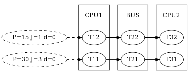
Base scenario

System Model¶

First, we create an empty system, which is just a container for all other objects:

    # generate an new system
    s = model.System('step1')

The next step is to create the three resources and bind them to the system via pycpa.model.System.bind_resource(). When creating a resource via pycpa.model.Resource(), the first argument of the constructor sets the resource id (a string) and the second defines the scheduling policy. The scheduling policy is defined by a reference to an instance of a scheduler class derived from pycpa.analysis.Scheduler. For SPP, this is pycpa.schedulers.SPPScheduler which we use for both processing resources. For the bus, we use pycpa.schedulers.SPNPScheduler.

    # add three resources (2 CPUs, 1 Bus) to the system
    # and register the SPP scheduler (and SPNP for the bus)
    r1 = s.bind_resource(model.Resource("CPU1", schedulers.SPPScheduler()))
    r2 = s.bind_resource(model.Resource("BUS",  schedulers.SPNPScheduler()))
    r3 = s.bind_resource(model.Resource("CPU2", schedulers.SPPScheduler()))

The next part is to create tasks and bind them to a resource via pycpa.model.Resource.bind_task(). For tasks, we pass some parameters to the constructor, namely the identifier (string), the scheduling_parameter, and the worst- and best-case execution times (wcet and bcet). The scheduling_parameter is evaluated by the scheduler which was assigned to the resource. For SPP and SPNP, it specifies the priority. By default higher numbers denote lower priorities.

    # create and bind tasks to r1
    t11 = r1.bind_task(model.Task("T11", wcet=10, bcet=5, scheduling_parameter=2))
    t12 = r1.bind_task(model.Task("T12", wcet=3, bcet=1, scheduling_parameter=3))

    # create and bind tasks to r2
    t21 = r2.bind_task(model.Task("T21", wcet=2, bcet=2, scheduling_parameter=2))
    t22 = r2.bind_task(model.Task("T22", wcet=9, bcet=5, scheduling_parameter=3))

    # create and bind tasks to r3
    t31 = r3.bind_task(model.Task("T31", wcet=5, bcet=3, scheduling_parameter=3))
    t32 = r3.bind_task(model.Task("T32", wcet=3, bcet=2, scheduling_parameter=2))

In case tasks communicate with each other through event propagation (e.g. one task fills the queue of another task), we model this through task links, which are created by pycpa.model.Task.link_dependent_task() A task link is abstract and does not consume any additional time. In case of communication-overhead it must be modeled by using other resources/tasks.

    # specify precedence constraints: T11 -> T21 -> T31; T12-> T22 -> T32
    t11.link_dependent_task(t21).link_dependent_task(t31)
    t12.link_dependent_task(t22).link_dependent_task(t32)

Last, we need to assign activation patterns (aka input event models) to the first tasks in the task chains, i.e. T11 and T12. We do this by assigning a periodic with jitter model, which is implemented by pycpa.model.PJdEventModel().

    # register a periodic with jitter event model for T11 and T12
    t11.in_event_model = model.PJdEventModel(P=30, J=3)
    t12.in_event_model = model.PJdEventModel(P=15, J=1)

Plotting the Task-Graph¶

After creating the system model, we can use pycpa.graph.graph_system() from the graph module in order to visualize the task graph. Here, we create a DOT (graphviz) and PDF file.

    # graph the system to visualize the architecture
    g = graph.graph_system(s, filename='%s.pdf' % s.name, dotout='%s.dot' % s.name, show=False, chains=chains)

Analysis¶

The analysis is performed by calling pycpa.analysis.analyze_system(). This will will find the fixed-point of the scheduling problem and terminate if a result was found or if the system is not feasible (e.g. one busy window or the amount a propagations was larger than a limit or a resource is overloaded).

    # perform the analysis
    print("\nPerforming analysis of system '%s'" % s.name)
    task_results = analysis.analyze_system(s)

pycpa.analysis.analyze_system() returns a dictionary with results for each task in the form of instances to pycpa.analysis.TaskResult. Finally, we print out the resulting worst-case response times and the corresponding details of the busy-window in which the worst-case response-time was found.

    # print the worst case response times (WCRTs)
    print("Result:")
    for r in sorted(s.resources, key=str):
        for t in sorted(r.tasks & set(task_results.keys()), key=str):
            print("%s: wcrt=%d" % (t.name, task_results[t].wcrt))
            print("    b_wcrt=%s" % (task_results[t].b_wcrt_str()))

The output of this example is:

pyCPA - Compositional Performance Analysis in Python.

Version 1.2
Copyright (C) 2010-2017, TU Braunschweig, Germany. All rights reserved.

Permission is hereby granted, free of charge, to any person obtaining a copy
of this software and associated documentation files (the "Software"), to deal
in the Software without restriction, including without limitation the rights
to use, copy, modify, merge, publish, distribute, sublicense, and/or sell
copies of the Software, and to permit persons to whom the Software is
furnished to do so, subject to the following conditions:

The above copyright notice and this permission notice shall be included in
all copies or substantial portions of the Software.

THE SOFTWARE IS PROVIDED "AS IS", WITHOUT WARRANTY OF ANY KIND, EXPRESS OR
IMPLIED, INCLUDING BUT NOT LIMITED TO THE WARRANTIES OF MERCHANTABILITY,
FITNESS FOR A PARTICULAR PURPOSE AND NONINFRINGEMENT. IN NO EVENT SHALL THE
AUTHORS OR COPYRIGHT HOLDERS BE LIABLE FOR ANY CLAIM, DAMAGES OR OTHER
LIABILITY, WHETHER IN AN ACTION OF CONTRACT, TORT OR OTHERWISE, ARISING FROM,
OUT OF OR IN CONNECTION WITH THE SOFTWARE OR THE USE OR OTHER DEALINGS IN
THE SOFTWARE.

invoked via: examples/tutorial.py

check_violations :       False 
debug            :       False 
e2e_improved     :       False 
max_iterations   :        1000 
max_wcrt         :         inf 
nocaching        :       False 
propagation      : busy_window 
show             :       False 
verbose          :       False 




Performing analysis of system 'step1'
Result:
T21: wcrt=11
    b_wcrt=blocker:9, q*WCET:1*2=2
T22: wcrt=11
    b_wcrt=T21:eta*WCET:1*2=2, blocker:0, q*WCET:1*9=9
T11: wcrt=10
    b_wcrt=q*WCET:1*10=10
T12: wcrt=13
    b_wcrt=T11:eta*WCET:1*10=10, q*WCET:1*3=3
T31: wcrt=11
    b_wcrt=T32:eta*WCET:2*3=6, q*WCET:1*5=5
T32: wcrt=3
    b_wcrt=q*WCET:1*3=3

As you can see, the worst-case response times of the tasks are 11, 11, 10, 13, 11 and 3. We can also see, that for T21, a lower-priority blocker (T22) has been accounted as required for SPNP scheduling.

End-to-End Path Latency Analysis¶

After the WCRT analysis, we can additionally calculate end-to-end latencies of task chains. For this, we first need to define pycpa.model.Path objects and bind them to the system via pycpa.model.System.bind_path(). A path is created from a name and a sequence of tasks. Note that, the tasks will be automatically linked according to the given sequence if the corresponding task links are not already registered.

    # specify paths
    p1 = s.bind_path(model.Path("P1", [t11, t21, t31]))
    p2 = s.bind_path(model.Path("P2", [t12, t22, t32]))

The path analysis is invoked by pycpa.path_analysis.end_to_end_latency() with the path to analysis, the task_results dictionary and the number of events. It returns the minimum and maximum time that it may take on the given path to process the given number of events.

    # perform path analysis of selected paths
    for p in paths:
        best_case_latency, worst_case_latency = path_analysis.end_to_end_latency(p, task_results, n=1)
        print("path %s e2e latency. best case: %d, worst case: %d" % (p.name, best_case_latency, worst_case_latency))

The corresponding output is:

path P1 e2e latency. best case: 10, worst case: 32
path P2 e2e latency. best case: 8, worst case: 27

Step 2: Refining the Analysis ¶

In this step, we show how analysis and propagation methods can be replaced in order to apply an improved analysis. More precisely, we want to exploit inter-event stream correlations that result from the SPNP scheduling on the bus as published in [Rox2010].

Refining the Analysis

System Model¶

We use the same system model as before but replace the scheduler on CPU2 by pycpa.schedulers.SPPSchedulerCorrelatedRox.

    r3.scheduler = schedulers.SPPSchedulerCorrelatedRox()

This scheduler exploits inter-event stream correlations that are accessed via the correlated_dmin() function of the input event models. It therefore requires this function to be present for all event models on this resource (CPU2). We achieve this by replacing the propagation method by pycpa.propagation.SPNPBusyWindowPropagationEventModel for alls tasks on the bus.

    for t in r2.tasks:
        t.OutEventModelClass = propagation.SPNPBusyWindowPropagationEventModel

This results in the following analysis output:

Performing analysis of system 'step2'
Result:
T21: wcrt=11
    b_wcrt=blocker:9, q*WCET:1*2=2
T22: wcrt=11
    b_wcrt=T21:eta*WCET:1*2=2, blocker:0, q*WCET:1*9=9
T11: wcrt=10
    b_wcrt=q*WCET:1*10=10
T12: wcrt=13
    b_wcrt=T11:eta*WCET:1*10=10, q*WCET:1*3=3
T31: wcrt=5
    b_wcrt=q*WCET:1*5=5
T32: wcrt=3
    b_wcrt=q*WCET:1*3=3
path P1 e2e latency. best case: 10, worst case: 26
path P2 e2e latency. best case: 8, worst case: 27

You can see that the WCRT of T31 improved from 11 to 5.

Step 3: Junctions and Forks ¶

In this step, we illustrate the use of junctions and forks. Junctions need to be inserted to allow combining multiple input event streams according to a given strategy. Forks can be used if a task has multiple dependent tasks (successors). A customized fork strategy can be used if different event models shall be propagated to these tasks (e.g. in case of hierarchical event streams [Rox2008]). In this example (see figure), we model the scenario that T12 and T13 produce data that is transmitted by the same bus message which is received by the RX task on CPU2. Depending on whether T12 or T13 issued the message, T32 or T33 will be activated respectively. Hence, junctions and forks enable modelling complex scenarios such as multiplexing and demultiplexing of messages as in [Thiele2015].

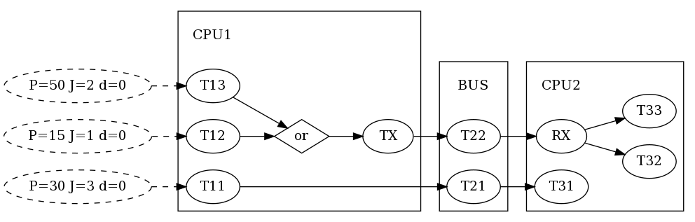
Junctions and forks

System Model¶

Again, we start with the same system model as presented in the base scenario but remove the dependencies between T12, T22 and T32 by resetting next_tasks attribute. Note that modifying a system model in such a way is not recommended but used for the sake of brevity in this tutorial.

    # remove links between t12, t22 and t32
    t12.next_tasks = set()
    t22.next_tasks = set()

Next, we add the additional tasks T31 and TX to CPU1 and specify an input event model for T31.

    # add one more task to R1 
    t13 = r1.bind_task(model.Task("T13", wcet=5, bcet=2, scheduling_parameter=4))
    t13.in_event_model = model.PJdEventModel(P=50, J=2)
    # add TX task on R1
    ttx = r1.bind_task(model.Task("TX", wcet=2, bcet=1, scheduling_parameter=1))

Now, we need a junction in order to combine the output event models of T12 and T13 into and provide the input event model of TX. This is achieved by registering a pycpa.model.Junction to the system via pycpa.model.System.bind_junction(). A junction is assigned a name and a strategy that derives from pycpa.analysis.JunctionStrategy. Some strategies are already defined in the pycpa.junctions module. Here, we use the pycpa.junctions.ORJoin in order to model that TX will be activated whenever T12 or T13 produce an output event.

    # add OR junction to system
    j1 = s.bind_junction(model.Junction(name="J1", strategy=junctions.ORJoin()))

Of course, we also need to add the corresponding task links.

    # link t12 and t13 to junction
    t12.link_dependent_task(j1)
    t13.link_dependent_task(j1)

    # link junction to tx
    j1.link_dependent_task(ttx)

On CPU2, we also need to add new tasks: T31 and RX. More specifically, we add RX as a pycpa.model.Fork which inherits from pycpa.model.Task. A fork also requires a strategy. Here, we use PathJitterForkStrategy that we explain later in Writing a Fork Strategy.

Before that, let us register the missing task links.

    # link rx to t32 and t33
    trx.link_dependent_task(t32)
    trx.link_dependent_task(t33)

    # link tx to t22 to rx
    ttx.link_dependent_task(t22).link_dependent_task(trx)

A fork also allows adding a mapping from its dependent tasks to for instance an identifier or an object that will be used by the fork strategy to distinguish the extracted event models. We use this in order to map the tasks T32 and T33 to T12 and T13 respectively.

    # map source and destination tasks (used by fork strategy)
    trx.map_task(t32, t12)
    trx.map_task(t33, t13)

Writing a Fork Strategy¶

In this example, we want to extract separate input event models for T32 and T33 as T32 (T33) will only be activated by messages from T12 (T13). This can be achieved by encapsulating several inner event streams into an outer (hierarchical) event streams as presented in [Rox2008]. Basically, the jitter that the outer event stream experiences can be applied to the inner event streams. Hence, we need to write a fork strategy that extract the inner (original) event streams before their combination by the junction and applies the path jitter that has been accumulated from the junction to the fork. A fork strategy must implement the function output_event_model() which returns the output event model for a given fork and one of its dependent tasks. Our fork strategy uses the previously specified mapping to get the corresponding source task (i.e. T12 and T13) and creates the path object via pycpa.util.get_path(). The jitter propagation is then implemented by inheriting from pycpa.propagation.JitterPropagationEventModel but using the path jitter (worst-case latency - best-case latency) instead of the response-time jitter (wcrt-bcrt).

    class PathJitterForkStrategy(object):

        class PathJitterPropagationEventModel(propagation.JitterPropagationEventModel):
            """ Derive an output event model from an in_event_model of the given task and
                the end-to-end jitter along the given path.
            """
            def __init__(self, task, task_results, path):
                self.task = task
                path_result = path_analysis.end_to_end_latency(path, task_results, 1)
                self.resp_jitter = path_result[1] - path_result[0]
                self.dmin = 0
                self.nonrecursive = True

                name = task.in_event_model.__description__ + "+J=" + \
                    str(self.resp_jitter) + ",dmin=" + str(self.dmin)

                model.EventModel.__init__(self,name,task.in_event_model.container)

                assert self.resp_jitter >= 0, 'response time jitter must be positive'

        def __init__(self):
            self.name = "Fork"

        def output_event_model(self, fork, dst_task, task_results):
            src_task = fork.get_mapping(dst_task)
            p = model.Path(src_task.name + " -> " + fork.name, util.get_path(src_task, fork))
            return PathJitterForkStrategy.PathJitterPropagationEventModel(src_task, task_results, p)

Analysis¶

When running the analysis, we obtain the following output:

Performing analysis of system 'step3'
Result:
T21: wcrt=11
    b_wcrt=blocker:9, q*WCET:1*2=2
T22: wcrt=11
    b_wcrt=T21:eta*WCET:1*2=2, blocker:0, q*WCET:1*9=9
T11: wcrt=20
    b_wcrt=TX:eta*WCET:5*2=10, q*WCET:1*10=10
T12: wcrt=26
    b_wcrt=T11:eta*WCET:2*10=20, TX:eta*WCET:7*2=14, q*WCET:2*3=6
T13: wcrt=55
    b_wcrt=T11:eta*WCET:2*10=20, T12:eta*WCET:4*3=12, TX:eta*WCET:9*2=18, q*WCET:1*5=5
TX: wcrt=6
    b_wcrt=q*WCET:4*2=8
RX: wcrt=2
    b_wcrt=q*WCET:1*2=2
T31: wcrt=43
    b_wcrt=RX:eta*WCET:9*2=18, T32:eta*WCET:6*3=18, q*WCET:2*5=10
T32: wcrt=15
    b_wcrt=RX:eta*WCET:3*2=6, q*WCET:3*3=9
T33: wcrt=76
    b_wcrt=RX:eta*WCET:11*2=22, T31:eta*WCET:4*5=20, T32:eta*WCET:8*3=24, q*WCET:2*5=10

Plotting Event Models¶

Now, we are interested in the event models that were extracted by the fork. For this, we use the pycpa.plot module to plot and compare the input event model of T12 and T32.

    plot_in = [t12, t32, ttx]

    # plot input event models of selected tasks
    for t in plot_in:
        plot.plot_event_model(t.in_event_model, 7, separate_plots=False, file_format='pdf', file_prefix='event-model-%s'
                % t.name, ticks_at_steps=False)

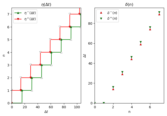
Input event model of T12.

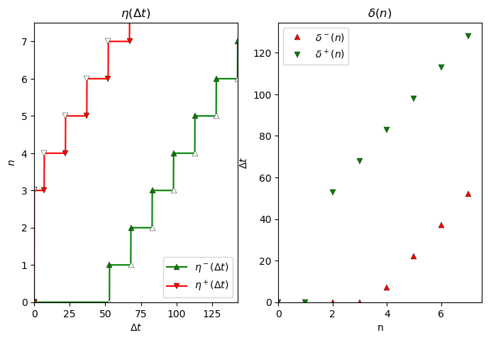
Input event model of T32.

Step 4: Cause-Effect Chains ¶

In this step, we demonstrate how we can compute end-to-end latencies for cause-effect chains. In contrast to a path, which describes an event stream across a chains of (dependent) tasks, a cause-effect chain describes a sequence of independently (time-)triggered tasks. In both cases, data is processed by a sequence of tasks but with different communication styles between the tasks.

Cause-Effect Chains

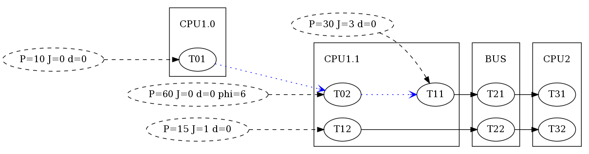
We modify the base scenario by moving from single-core CPUs to multiple cores per CPU. More precisely, we added one core to CPU1 as illustrated in the figure to the right:

    r1.name = 'CPU1.1'
    r10 = s.bind_resource(model.Resource("CPU1.0", schedulers.SPPScheduler()))

We also a new task to both cores:

    t01 = r10.bind_task(model.Task("T01", wcet=5, bcet=2, scheduling_parameter=1))
    t02 =  r1.bind_task(model.Task("T02", wcet=5, bcet=2, scheduling_parameter=4))

    t01.in_event_model = model.PJdEventModel(P=10, phi=0)
    t02.in_event_model = model.PJdEventModel(P=60, phi=6)

    t01 = r10.bind_task(model.Task("T01", wcet=5, bcet=2, scheduling_parameter=1))
    t02 =  r1.bind_task(model.Task("T02", wcet=5, bcet=2, scheduling_parameter=4))

    t01.in_event_model = model.PJdEventModel(P=10, phi=0)
    t02.in_event_model = model.PJdEventModel(P=60, phi=6)

Now we define an effect chain comprising T01, T02 and T11.

    chains = [ model.EffectChain(name='Chain1', tasks=[t01, t02, t11]) ]

Note that every task in the effect chain has its own periodic input event model. In contrast to activation dependencies (solid black arrows in the figure), the data dependencies within the effect chain are illustrated by blue dotted arrows.

Analysis¶

The effect chain analysis is performed similar to the path analysis. Note that there are two different latency semantics: reaction time and data age. Here, we are interested in the data age.

    # perform effect-chain analysis
    for c in chains:
        details = dict()
        data_age = path_analysis.cause_effect_chain_data_age(c, task_results, details)
        print("chain %s data age: %d" % (c.name, data_age))
        print("  %s" % str(details))

When running the analysis, we obtain the following output:

Performing analysis of system 'step4'
Result:
T21: wcrt=11
    b_wcrt=blocker:9, q*WCET:1*2=2
T22: wcrt=11
    b_wcrt=T21:eta*WCET:1*2=2, blocker:0, q*WCET:1*9=9
T01: wcrt=5
    b_wcrt=q*WCET:1*5=5
T02: wcrt=21
    b_wcrt=T11:eta*WCET:1*10=10, T12:eta*WCET:2*3=6, q*WCET:1*5=5
T11: wcrt=10
    b_wcrt=q*WCET:1*10=10
T12: wcrt=13
    b_wcrt=T11:eta*WCET:1*10=10, q*WCET:1*3=3
T31: wcrt=11
    b_wcrt=T32:eta*WCET:2*3=6, q*WCET:1*5=5
T32: wcrt=3
    b_wcrt=q*WCET:1*3=3
path P1 e2e latency. best case: 10, worst case: 32
path P2 e2e latency. best case: 8, worst case: 27
chain Chain1 data age: 116
  {'T01-PHI+J': 0, 'T01-T02-delay': 23, 'T01-WCRT': 5, 'T02-T11-delay': 57, 'T02-WCRT': 21, 'T11-WCRT': 10}

Step 5: Complex Run-Time Environments ¶

It has been shown that CPA may provide very conservative results if a lot of task dependencies are present on a single resource [Schlatow2016]. The general idea to mitigate this is to only use event model propagation at resource boundaries as illustrated in the figure to the right. On the resource itself, we end up with task chains that can be analysed as a whole with the busy-window approach (see [Schlatow2016], [Schlatow2017]).

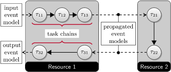
Task Chains

The implementation of this approach is available as an extension to the pyCPA core at https://github.com/IDA-TUBS/pycpa_taskchain. It replaces the pycpa.model.Resource with a TaskchainResource and also the Scheduler with an appropriate implementation.

Hence, we need to import the modules as follows:

        from taskchain import model as tc_model
        from taskchain import schedulers as tc_schedulers

We then model the scenario depicted in the figure as follows:

    s = model.System(name='step5')

    # add two resources (CPUs) to the system
    # and register the static priority preemptive scheduler
    r1 = s.bind_resource(tc_model.TaskchainResource("Resource 1", tc_schedulers.SPPSchedulerSync()))
    r2 = s.bind_resource(tc_model.TaskchainResource("Resource 2", tc_schedulers.SPPSchedulerSync()))

    # create and bind tasks to r1
    t11 = r1.bind_task(model.Task("T11", wcet=10, bcet=1, scheduling_parameter=1))
    t12 = r1.bind_task(model.Task("T12", wcet=2, bcet=2, scheduling_parameter=3))
    t13 = r1.bind_task(model.Task("T13", wcet=4, bcet=2, scheduling_parameter=6))

    t31 = r1.bind_task(model.Task("T31", wcet=5, bcet=3, scheduling_parameter=4))
    t32 = r1.bind_task(model.Task("T32", wcet=5, bcet=3, scheduling_parameter=2))

    t21 = r2.bind_task(model.Task("T21", wcet=3, bcet=1, scheduling_parameter=2))
    t22 = r2.bind_task(model.Task("T22", wcet=9, bcet=4, scheduling_parameter=2))

    # specify precedence constraints
    t11.link_dependent_task(t12).link_dependent_task(t13).link_dependent_task(t21).\
            link_dependent_task(t22).link_dependent_task(t31).link_dependent_task(t32)

    # register a periodic with jitter event model for T11
    t11.in_event_model = model.PJdEventModel(P=50, J=5)

    # register task chains
    c1 = r1.bind_taskchain(tc_model.Taskchain("C1", [t11, t12, t13]))
    c2 = r2.bind_taskchain(tc_model.Taskchain("C2", [t21, t22]))
    c3 = r1.bind_taskchain(tc_model.Taskchain("C3", [t31, t32]))

    # register a path
    s1 = s.bind_path(model.Path("S1", [t11, t12, t13, t21, t22, t31, t32]))

When running the analysis, we get the task-chain response time results as the results for the last task in each chain:

Performing analysis of system 'step5'
Result:
T13: wcrt=26
    b_wcrt=T11:q*WCET:1*10=10, T12:q*WCET:1*2=2, T13:q*WCET:1*4=4, T31:eta*WCET:1*5=5, T32:eta*WCET:1*5=5
T32: wcrt=22
    b_wcrt=T11:WCET:10, T12:WCET:2, T31:q*WCET:1*5=5, T32:q*WCET:1*5=5
T22: wcrt=12
    b_wcrt=T21:q*WCET:1*3=3, T22:q*WCET:1*9=9
Warning: no task_results for task T11
Warning: no task_results for task T12
Warning: no task_results for task T21
Warning: no task_results for task T31
path S1 e2e latency. best case: 16, worst case: 60

Tutorial¶

Introduction¶

Initialization¶

Step 1: Base Scenario¶

System Model¶

Plotting the Task-Graph¶

Analysis¶

End-to-End Path Latency Analysis¶

Step 2: Refining the Analysis¶

System Model¶

Step 3: Junctions and Forks¶

System Model¶

Writing a Fork Strategy¶

Analysis¶

Plotting Event Models¶

Step 4: Cause-Effect Chains¶

Analysis¶

Step 5: Complex Run-Time Environments¶

Introduction ¶

Initialization ¶

Step 1: Base Scenario ¶

Step 2: Refining the Analysis ¶

Step 3: Junctions and Forks ¶

Step 4: Cause-Effect Chains ¶

Step 5: Complex Run-Time Environments ¶